How to write a statistical analysis paper: Step 4
We’ve looked at data on Body Mass Index (BMI) by race. Now let’s take a look at our sample another way. Instead of using BMI as a variable, let’s use obesity as a dichotomous variable, defined as a BMI greater than 30. It just so happened (really) that this variable was already in the data set so I didn’t even need to create it.
The code is super-simple and shown below. The reserved SAS keywords are capitalized just to make it easier to spot what must remain the same. Let’s look at this line by line
LIBNAME mydata “/courses/some123/c_1234/” ACCESS=READONLY;
PROC FREQ DATA = mydata.coh602 ;
TABLES race*obese / CHISQ ;
WHERE race NE “” ;
RUN ;
LIBNAME mydata “/courses/some123/c_1234/” ACCESS=READONLY;
Identifies the directory where the data for your course are stored. As a student, you only have read access.
PROC FREQ DATA = mydata.coh602 ;
Begins the frequency procedure, using the data set in the directory linked with mydata in the previous statement.
TABLES race*obese / CHISQ ;
Creates a cross-tabulation of race by obesity and the CHISQ following the option statistic produces the second table you see below of chi-square and other statistics that test the hypothesis of a relationship between two categorical variables.
WHERE race NE “” ;
Only selects those observations where we have a value for race (where race is not equal to missing)
RUN ;
Pretty obvious? Runs the program.
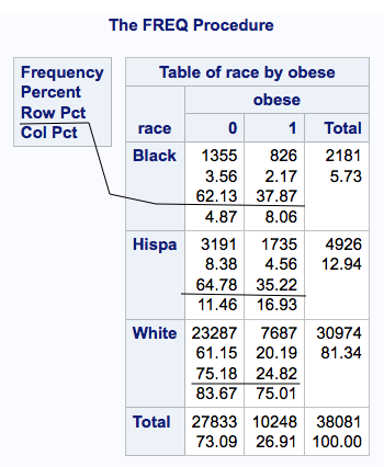
Similar to our ANOVA results previously, we see that the obesity rates for black and Hispanic samples are similar at 35% and 38% while the proportion of the white population that is obese is 25%. These numbers are the percentage for each row. As is standard practice, a 0 for obesity means no, the respondent is not obese and a 1 means yes, the person is obese.
The CHISQ option produces the table below. The first three statistics are all tests of statistical significance of the relationship between the two variables. 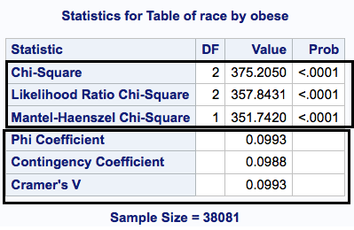
You can see from this that there is a statistically significant relationship between race and obesity. Another way to phrase this might be that the distribution of obesity is not the same across races.
The next three statistics give you the size of the relationship. A value of 1.0 denotes perfect agreement (be suspicious if you find that, it’s more often you coded something wrong than that everyone of one race is different from everyone of another race). A value of 0 indicates no relationship whatsoever between the two variables. Phi and Cramer’s V range from -1 to +1 , while the contingency coefficient ranges from 0 to 1. The latter seems more reasonable to me since what does a “negative” relationship between two categorical variables really mean? Nothing.
From this you can conclude that the relationship between obesity and race is not zero and that it is a fairly small relationship.
Next, I’d like to look at the odds ratios and also include some multivariate analyses. However, I’m still sick and some idiot hit my brand new car on the freeway yesterday and sped off, so I am both sick and annoyed. So … I’m going back to bed and discussion of the next analyses will have to wait until tomorrow.