A quick introduction to interpretation of Exploratory Factor Analysis: Mplus Example
Last week I wrote a bit about how to get an exploratory factor analysis using Mplus. The question now, is what does that output MEAN ?
First, you just get some information on the programming statements or defaults that produced your output:
INPUT READING TERMINATED NORMALLY
Exploratory Factor Analysis ;
SUMMARY OF ANALYSIS
Number of groups 1
Number of observations 730
Number of dependent variables 6
Number of independent variables 0
Number of continuous latent variables 0
Observed dependent variables
Continuous
Q1F1 Q2F1 Q3F1 Q1F2 Q2F2 Q3F2
Estimator ML
Rotation GEOMIN
Row standardization CORRELATION
Type of rotation OBLIQUE
This tells us we our analyzing all of the data as one group, and not, for example, separate analyses for males and females. We have 730 records, six variables, all of which are continuous and listed above. The maximum likelihood method (ML) of estimation is used and the default rotation, GEOMIN, which is an oblique method, that is it allows the factors to be correlated.
Here we have a list of our eigenvalues
RESULTS FOR EXPLORATORY FACTOR ANALYSIS
EIGENVALUES FOR SAMPLE CORRELATION MATRIX
1 ……… 2 ……… 3 4 5
________ ________ _____ ________ ________
1.866 1.262 0.866 0.750 0.716
EIGENVALUES FOR SAMPLE CORRELATION MATRIX
6
________
0.539
In this case, you could go ahead with the eigenvalue greater than one rule, but let’s take a look at a couple of other statistics. First, we have the results from the one factor solution. Here we have the chi-square testing the goodness of fit of the model
Chi-Square Test of Model Fit
Value 96.228
Degrees of Freedom 9
P-Value 0.0000
We want this test to be non-significant because our null hypothesis is there is no difference between the observed data and our hypothesized one-factor model. This null is soundly rejected.
Let’s take a look at the Chi-square for our two-factor solution
Chi-Square Test of Model Fit
Value 3.016
Degrees of Freedom 4
P-Value 0.5552
You can clearly see that the chi-square is much smaller and non-significant.
Let’s take a look at two other tests. The Root Mean Square Error of Approximation (RMSEA) for the one-factor solution is .115, as shown below. We would like to see an RMSEA less than .05 which is clearly not the case here.
RMSEA (Root Mean Square Error Of Approximation)
Estimate 0.115
90 Percent C.I. 0.095 0.137
Probability RMSEA <= .05 0.000
For the two factor solution, our RMSEA rounds to zero, as shown below
RMSEA (Root Mean Square Error Of Approximation)
Estimate 0.000
90 Percent C.I. 0.000 0.049
Probability RMSEA <= .05 0.954
Clearly, we are liking the two-factor solution here, yes? The eigenvalue > 1 rule (which should not be TOO emphasized) points there, as does the model fit chi-square and the RMSEA.
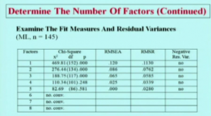
In their course on factor analysis, Muthen & Muthen give this very nice example of a table comparing different factor solutions using the data
They also like the scree plot, which I do, too. I also agree with them that one should never blindly follow some rule but rather have some theory or expectation about how the factors should fall out. I also agree with them in looking at multiple indicators, for example, scree plot, chi-square, RMSEA and eigen-values.

i would like to continue on the same topic of data output interpretation by EFA<CFA and SEM model and if you have such example on interpretation i would love to have it urgently