May

3

I had more than the two tips on becoming a better programmer than I gave in the last post but I had run out of margarita. Now, being replenished with tequila and fresh lime by The Invisible Developer, here are two more. He often tells me that I should refer to myself as a developer and not a programmer because that is beneath me. I have never pretended to be cool. I started with punched cards as a programmer and a programmer I will remain. At least until the second margarita.

margarita
It’s Friday!

If you aren’t familiar with github, you could have gone to Chris Hemedinger’s super demo at SAS Global Forum. We use github for version control and it is indispensable for that. When you have several people working on the same program, I can edit files, you can, too, and we all upload and download the latest versions without copying over each other’s code. If you are on a project with more than one developer, once you have used a git repository, you’ll fight anyone who tries to take it away.

Because it is so good for sharing, github is used a lot for open source projects and for people just making their code publicly available.

The main thing I learned that I didn’t know is that there is a https://github.com/sassoftware

I had just assumed since SAS is a private company and definitely not open source that there would not be much available. I was wrong.

Whatever language you use, there is probably a github for it.

Here is a funny thing. When I first started learning JavaScript, I scavenged github to find examples of people making simple games like tic-tac-toe , Memory or mazes. I’d modify the code to do what I wanted and I thought all of these people were so much smarter than me.

After I learned a bit more, sometimes I saw functions or libraries in the code that didn’t do anything and I realized that a lot of these people had done the exact same thing as me – copied someone else’s code and modified it for their purposes.

Start by copying code from github, but don’t stop there

If you ask me – and even if you don’t, I’m going to tell you anyway – it is absolutely fine to download code from someone else’s repository on github and tweak it a little for your own purposes. However, don’t stop there! Dive into it. Figure out what each function does, try to understand their logic.

A better person than me would have their own public git repository. Oh well, I have a bucket of private ones for work and I’ve been writing this blog for 11 years, so that will have to do. YOU should definitely have public repository, though. Changing the subject here …

Git Repositories that are NOT python, R or Viya

The top repositories almost all entail either integrating SAS and Python (not surprising because it is open source) or Viya or Visual Analytics (presumably because it is expensive and SAS wants to promote it). There are also a smattering of SAS-and-R repositories in the top hits and repositories for SAS and iOS and SAS and Android. I’m not interested in any of that at the moment.

Right now, I am super-swamped but I should have some free time over the summer, so here are my personal interests I am marking for later. With 116 repositories, any SAS aficionado should find something of interest, and remember, this is just the sassoftware repository. There are additional repositories of individual users, like the last one I noted below

SAS Studio Tasks is an area I’d like to learn more about, as in writing your own custom tasks.

Data mining is an area I am ALWAYS wanting to brush up on more . This library of flow diagrams for specific data mining topics looks really cool.

Not a SAS Institute repository, this one from Michael Friendly is on macros and looks super cool.

As I mentioned above, I started using github for JavaScript code and there are TONS of repositories for just about any language that would tickle your fancy (what exactly IS a fancy, anyway?)

I have more tips but it will have to wait for another margarita and since my grandchildren are spending the weekend and just invaded my office, that will have to wait.

Apr

29

I did a random sample of presentations at SAS Global Forum today, if random is defined as of interest to me, which let’s be honest, is pretty damn random most of the time. 

Tip #1 Stalk Interesting People

I don’t mean in a creepy showing up at their hotel room way. If you see someone presenting either in person or referenced in twitter, blogs, etc. , check out what else that person has freely available on the web, in published proceedings, etc.

Let me give you an example that applies even if you are not into logistic regression. (You’re not? Feel shame.)

The first session I attended was a Super Demo in the exhibit hall which for some reason I don’t understand is always called the Quad. 

In a nutshell, logistic regression is usually 

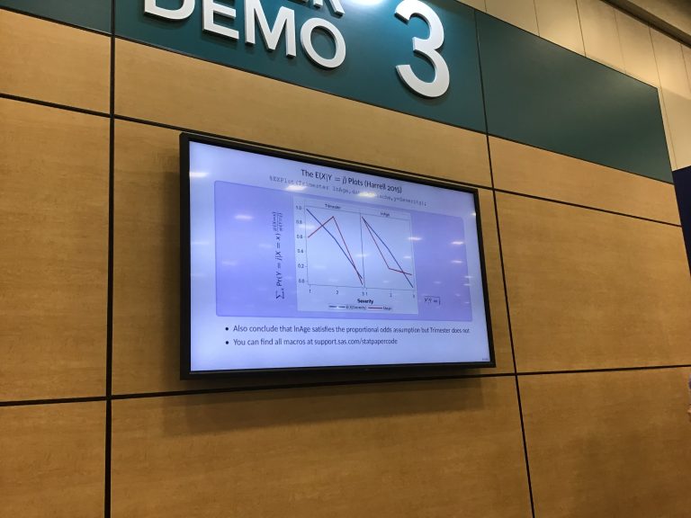
What if the data fit the proportional odds model for some of the explanatory variables and not others? You can do a partial proportional odds model. 

Line plots on slide
Graphing your data is a great way to see if the proportional odds model makes sense. You can see that it does for the variable on the right, but for the left, not so much.

Unfortunately, the super demos do not have a paper published in the app or proceedings, however, the presenter, Bob Derr from SAS mentioned he had presented a paper on this topic in 2013 (way to play hard to get, Bob – not!)

Paper reference on slide (also below in blog)

I skipped the next presentation to read it (and to write this post). If you are at all interested in multinomial and ordinal logistic regression, you should, too. You can find it here in the SAS Global Forum 2103 proceedings. http://support.sas.com/resources/papers/proceedings13/446-2013.pdf

It’s an outstanding paper and I am going to require it for my course next year. I think the students will find it far more accessible than some of the readings we have been using. They don’t complain loudly, but I know, I know. 

Tip #2 Read the Documentation (No, seriously, keep reading)

People who answer comments with LMGTFY (let me Google that for you) or RTFM (read the fucking manual), just so you know, that quit being funny around 1990. However, SAS documentation really is a treasure trove. It’s not just SAS, the same could be said about jQuery documentation or the WordPress Codex but we’re not talking about those today, are we? Please try to stay on topic. 

The SAS documentation runs many, many thousands of pages. It’s far better and more detailed than you would think. Let me give you an example a very helpful person named Michael pointed out in the Quad (what the hell is it with that name?) today. As I’ve mentioned several times lately, my students often struggle with repeated measures ANOVA. He suggested checking out the page on longitudinal data analysis.

http://support.sas.com/rnd/app/stat/procedures/LongitudinalAnalysis.html

It gives four different procedures (none of which are GLM, I noted, but that’s a discussion for another day). 

Related to that, I recommend when you are learning procedures just running some of the code examples. For example, here is one for repeated measures with PROC MIXED. http://documentation.sas.com/?docsetId=statug&docsetTarget=statug_mixed_examples02.htm&docsetVersion=15.1&locale=en. (Yes, I really do have that on my mind lately)

Think about this, though. Once you graduate from whatever your last degree turns out to be, you don’t have anyone checking your work and telling you if it is right or not. You just write your code and hope for the best. That sucks, huh?

When you are learning a new procedure, you can write code using the data shown in the SAS documentation and see if your results match. Like an answer key for life! I always wanted one of those.

Apr

25

Since the last few posts detailed errors in repeated measures with PROC GLM , I thought I should acknowledge that people seem to struggle just as much with PROC MIXED.

Forgetting data needs to be multiple rows

This is one of the first points of confusion for students. When you do a PROC MIXED, you need multiple records for each person. So, thinking back to my previous example with three time points, with PROC MIXED, and two options for treatment, my dataset needs to look like this:

SubjectExamTreatmentScore
1PreTalk43
1PostTalk46
1FollowTalk45
2PreDrug39

With GLM, you’d have 3 variables, named Pre, Post and Follow, for example (you *did* read the last post, right?). In PROC MIXED, your dataset has to be structured so that you have one variable, in this case, named “exam”, and it takes on one of three possible values.

Let’s start with the simplest case. I’d like to know, just like before, if there was a change from pre to post-test and if it was maintained at follow-up. In other words, my question is, “Was there a difference between the pretest and post-test and a difference between pretest and follow-up six months later?” I am not particularly interested in the post-test/ followup difference as such. Here is one way to code it:

Proc mixed data = example ;
class subject exam;
model score = exam ;
random subject ;
contrast “pre vs post” exam 1 -1 0 ;
contrast “pre vs follow” exam 1 0 -1 ;


The PROC GLM code from this post will give you the exact same results as the code above, but only if you have your data structured so that you have three variables instead of three records for each person.

I have a lot to say about CONTRAST statements, which I love, and random effects, about which I am neutral, and nested effects, that are not relevant to this example but could be. However, I am trying to not work past 9 pm and it’s already an hour later so … until next time.

Also, if you’re at SAS Global Forum, be sure to meet up and say “Hey!”

This is my day job …

Check it out. I make games that teach math, including, of course, statistics. Play AzTech: Meet the Maya – the only statistics game with Honduran fruit bats.

Apr

17

As I said in my last post, repeated measures ANOVA seems to be one of the procedures that confuses students the most. Let’s go through two ways to do an analysis correctly and the most common mistakes.

Our first example has people given an exam three times, a pretest, a posttest and a follow up and we want to see if the pretest differs from the other two time points.

proc glm data = example ;
model pre post follow = /nouni ;
repeated exams 3 contrast (1) /summary printm ;

Among other things, this will give you a table of Type III Sum of Squares that tells you that you have a significant difference across time. It will also give you contrasts between the 1st treatment and each of the other two.

You can see all of the output produced here.

This is using PROC GLM and so it requires that you have multiple VARIABLES representing each of the multiple times you measured people. This is in contrast to PROC MIXED which requires multiple records for each subject. We’ll get into that another day.

One thing that throws people all of the time is they ask, “Where did you get the exams variable?” In fact, I could have used any valid SAS name. It could have been “Nancy” instead of “exams” and that would have worked just as well. It’s a label we use for the factor measured multiple times. So, as counterintuitive as it sounds, there is NO variable named “exams” in your data set.

Let’s try a different example. This time, I have a treatment variable. I have administered two different treatments to my subjects. I want to see if treatment has any effect on improvement.

proc glm data =example ;
class treatment ;
model pre post follow = treatment/ nouni ;
repeated exams 3 /summary ;

The fixed effect does *not* go in your REPEATED statement

In this case, I do need a CLASS statement to specify my fixed effect of treatment. A really common mistake that students make is to code the REPEATED statement like this:

repeated treatment 3 /summary ; *WRONG! ;

It seems logical, right? Why would you use a completely made up name instead of one of your variables? If you think about it for a minute, though, treatment wasn’t repeated. Each subject only received one type of treatment.

When you are asking whether one group improved more than the other(s) what you are asking is, “Is there an interaction effect?” You can see by the table of Type III Sums of Squares produced below that there was no interaction effect.


A significant effect for the repeated measure does not mean your treatment worked!

A common mistake is to look at the significance for the repeated measure and because a significant change was found between times 1 and 3 to say that the treatment had an effect. In fact, though, we can see by the non-significant interaction effect that there was not an impact of treatment because there was no difference in the change in exam scores across the levels of treatment.

There are a lot of other common mistakes but I need to go back to work so those will have to wait for another blog.

Apr

14

When I teach students how to use SAS to do a repeated measures Analysis of Variance, it almost seems like those crazy foreign language majors I knew in college who were learning Portuguese and Italian at the same time.

I teach how to do a repeated measures ANOVA using both PROC GLM and PROC MIXED. It seems very likely in their careers my students will run into both general linear models and mixed models. The problem is that they confuse the two and the result is buggy code.

Let’s start with mistakes in PROC GLM today. Next time we can discuss mistakes in PROC MIXED.

Let’s say I have the simplest possible analysis – I’ve given the same students a pre- and a post-test and want to see if there has been a significant increase from time one to time two.

This will work just fine:

proc glm data =mydata.fl_pre_post ;
model pretest posttest = /nouni ;
repeated time 2 ;

Coding the repeated statement like this will also work

repeated time 2 (1 2) ;

So will

repeated time ;

It almost seems as if anything or nothing after the variable name will work. That’s not true. First of all,

repeated time 2 (a b) ; IS WRONG

… and will give you an error – Syntax error, expecting one of the following: a numeric constant, a datetime constant.

“Levels gives the number of levels associated with the factor being defined. When there is only one within-subject factor, the number of levels is equal to the number of dependent variables. In this case, levels is optional. When more than one within-subject factor is defined, however, levels is required,”

SAS 9.2 Users Guide

So, this explains why you can be happily using your repeated statement without bothering to specify the number of levels for a factor and then one day it doesn’t work. WHY? Because now you have two within-subject factors and you need to specify the number of levels but you don’t know that. This is why, when teaching I always include the number of levels. It will never cause your program to fail, even if it is unnecessary sometimes.

One more cool thing about the repeated statement for PROC GLM, you can do a planned contrast super easy. Let’s say I have done 3 tests, a pretest, a post-test and a follow-up. I want to compare the posttest and followup to the pretest.

proc glm data =mydata.fl_tests ;
model pretest posttest follow = /nouni ;
repeated test_time 3 contrast (1) /summary ;

What this will do is compare each of the other time points to the first one. A common mistake students make is to use a CONTRAST statement here with test_time. This will NOT work, although it will work with PROC MIXED, but that is a story for another day.

Jan

20

I was going to write more about reading JSON data but that will have to wait because I’m teaching a biostatistics class and I think this will be helpful to them.

What’s a codebook?

If you are using even a moderately complex data set, you will want a code book. At a minimum, it will tell you the name of each variable, the type (character, numeric or date), a label, if it has one and its position in the data set. It will also tell you the number of records and number of variables in a data set. In SAS, you can get all of this by running a PROC CONTENTS. (Also from a PROC DATASETS but we don’t cover that procedure in this class.)

So, for the sashelp.heart data set, for example, you would see:

output from Proc contents

The variable AgeAtDeath is the 12th variable in the data set. It is numeric, with a length of 8 and the label for it is “Age At Death”. Because it is a numeric variable, if you try to use it for any character functions, like finding a substring, you will get an error. (A substring is a subset of a string, so ‘ABC’ is a substring of ‘ABCDE’.)

Similarly, BP_Status is the 15th variable in the data set, it is a character, with a length of 7 and a label of “Blood Pressure Status”. Because it’s a character variable, if you try to do any procedures or functions that expect numeric variables, like find the mean, you will get an error. The label will be used in output, like in the table below.

Frequency distribution of blood pressure status

This is useful because you may have no idea what BP_Status is supposed to mean. HOWEVER, if you use “Blood Pressure Status” in your statements like the example below, you will get an error.

**** WRONG!!!
Proc means data=sashelp.heart ;
Var blood pressure status ;

Seems unfair, but that’s the way it is.

The above statement will assume you want the means for three separate variables named “blood” “pressure” and “status”.

There are no variables in the data set named “blood” or “pressure” so you will get an error. There is a variable named “status”, but it’s something completely different, a variable telling if the subject is alive or dead.

Even if you don’t have a real codebook available, you should at a minimum start any analysis by doing a PROC CONTENTS so you have the correct variable names and types.

What about these errors I was talking about, though? Where will you see them?

LOOK AT YOUR SAS LOG!!

If you are using SAS Studio , it’s the second tab in the middle window, to the right of the tab that says CODE.

Click on that tab and if you have any SYNTAX errors, they will conveniently show up in red.

Also, if you are taking a course and want help from your professor or a classmate, the easiest way for them to help you is if you is to copy and paste your SAS log into an email, or even better, download it and send it as an attachment.

Just because you have no errors in the SAS log doesn’t mean everything is all good, but it’s always the first place you should look.

To get a table of blood pressure status, you may have typed something like

Proc freq data=sashelp.heart ;
Tables status ;

That will run without errors but it will give you a table that gives status as alive or dead, not blood pressure as high, normal or optimal.

PROC CONTENTS is a sort of “codebook light”. A real codebook should also include the mean, minimum, maximum and more for each variable. We’ll talk about that in the next post. Or, who knows, maybe I’ll finally finish talking about reading in JSON data.

Jan

2

Sometimes data changes shape and type over time. In my case, we had a game that was given away free as a demo. We saved the player’s game state – that is, the number of points they had, objects they had earned in the game, etc. as a JSON object. Happy Day! The game became popular. Schools started using it. We came out with a premium version with lots more activities, a bilingual Spanish-English version, a bilingual Lakota- English version. Life is good.

Making Camp Premium on Google Play 

Once schools started using our games, they wanted data on how much students played, how many problems they answered. This is when life started to get complicated. We added more fields to the JSON object to show which activities they had completed and whether they had won.

Data for one person might look like this, or much, much longer.

“{“”points””:””8″”,””first_trade””:””false””,””first_visit””:””true””, “”has_wigwam””:””true””,””inventory””:””6,3,4,14″”,””inventory_position””:””[{\””left\””:0,\””top\””:0},{\””left\””:0,\””top\””:0},{\””left\””:0,\””top\””:0},{\””left\””:176,\””top\””:4},{\””left\””:-309,\””top\””:-254},{\””left\””:0,\””top\””:0},{\””left\””:619,\””top\””:-45},{\””left\””:0,\””top\””:0},{\””left\””:0,\””top\””:0},{\””left\””:0,\””top\””:0},{\””left\””:0,\””top\””:0},{\””left\””:0,\””top\””:0},{\””left\””:0,\””top\””:0},{\””left\””:0,\””top\””:0},{\””left\””:293,\””top\””:-44},{\””left\””:0,\””top\””:0},{\””left\””:0,\””top\””:0},{\””left\””:0,\””top\””:0},{\””left\””:0,\””top\””:0},{\””left\””:0,\””top\””:0},{\””left\””:0,\””top\””:0},{\””left\””:0,\””top\””:0}]””,””milestone””:””EarnPage””}”

The JSON engine didn’t work (not surprisingly)

I actually didn’t expect it would work because we didn’t actually have a JSON object but rather a JSON object converted to a string and saved in an SQL database. However, if something would only take a minute, I try it first

libname testmcb JSON fileref =reffile ;

Okay, so what now? We have a variable record length, the values we want might be in any column. It must be really difficult to figure out, right? Not really.

This next bit looks complicated but it actually took very little time to code. Before we get into the code, let’s talk about what I needed to do and why. The “why” is that I want to know how much kids played the games. There are three milestones – logging in, getting a wigwam and trading for items. However, some kids just liked playing the mini-games and they played A LOT without pausing to trade in their points. Also, you can’t just look at how many points they have because they may have traded some points for items. Fortunately, all items cost two points, so I need to compute points + (items in inventory/2).

This actually took me very little time. Let’s look at it bit by bit (ha ha).

The first line just assigns a file reference for where my text file is located.

FILENAME reffile '/home/annmaria.demars/data_analysis_examples/data2018/exceldata/mc_bilingualtest.txt';

Data mcb_json ;
INFILE reffile DLM="," LRECL = 1337 ;

*** READ IN FILE, VARIABLES ARE SEPARATED (DELIMITED) BY A COMMA. LENGTH OF THE RECORD IS 1,337 ;

INFORMAT first_trade $40. first_visit $40. has_wigwam $40. ;
INPUT  firstcol $ 15-16 @@ ;
IF firstcol = '":' THEN  INPUT @43 points $ first_trade $ first_visit $ has_wigwam $ ;
ELSE INPUT @15 points $ first_trade  first_visit  has_wigwam  ;

***** READ IN THE VARIABLES FOR TRADING, FIRST VISIT AND WIGWAM AS CHARACTER WITH A LENGTH OF 40 ;
****  READ COLUMNS 15-16 AND STAY ON THAT LINE ;
**** IF THE VALUE IN COLUMNS 15-16 = “:  THEN IT HAD MILESTONE AT THE BEGINNING;
***** THE VARIABLES WE WANT START AT COLUMN 43, OTHERWISE, THEY START AT COLUMN 15;
*** THESE ARE SEPARATED BY COMMAS SO WE CAN JUST LIST THE VARIABLE NAMES;
*** NOTE THAT I NEED TO SPECIFY THAT POINTS IS CHARACTER DATA SINCE IT’S NOT IN MY INFORMAT STATEMENT ;

IF INDEX(first_trade,"true") > 0 or index(first_trade,"1") > 0 then traded =0 ;
ELSE IF INDEX(first_trade,"false") or index(first_trade,"0") then traded =1 ;
IF INDEX(first_visit,"false") or index(first_visit,"0") then play_twice = 1 ;
ELSE IF INDEX(first_visit,"true") or index(first_visit,"null") or index(first_visit,"1") then play_twice = 0 ;
IF INDEX(has_wigwam,"true") then wigwam = 1 ;
ELSE IF INDEX(has_wigwam,"null") > 0 or index(has_wigwam,"0") > 0 then wigwam = 0 ;

*** ABOVE I JUST USE A FEW IF THEN STATEMENTS TO CREATE MY NEW VARIABLES ;
**** The INDEX function returns the position in the variable in the first argument where it finds the value in the second argument;
**** If the value isn’t found, it returns a value of 0 ;

This last step isn’t strictly necessary, except that it is. Here I do a cross-tabulation to make sure that all of the variables were assigned correctly and they were.  For example, you can see that if the value of “has_wigwam” was 0 or null the wigwam variable was set to 0. If has_wigwam was equal to “true” the wigwam variable was set to 1.

PROC FREQ ;
TABLES  traded*first_trade first_visit*play_twice wigwam*has_wigwam ;

Screen shot of table of has_wigwam by wigwam values

This would have worked for the whole JSON object except for the commas in the inventory. If you look at just a piece of the data, you can see that after the variables denoting milestones there is a variable that is actually an array, separated by commas.

“first_visit””:””true””, “”has_wigwam””:””true””,””inventory””:””6,3,4,14″”,”

We’ll look at how to handle that in the next post.

Dec

30

When I was young and knew everything, I would frequently see procedures or statistics and think, “When am I ever going to use THAT?” That was my thought when I learned about this new procedure to transpose a data set. (It was new then. Keep in mind, I learned SAS when I was pregnant with my first child. She is now CEO of a an educational game company and the mother of three children. )

PROC TRANSPOSE is super-useful. You might only think it is useful for transforming data for use with PROC GLM to use with PROC MIXED, or you might have no idea what the hell that means and it is still super-useful.

Let me give you today’s example. I’m looking for data to use in a biostatistics class I’m teaching next month. It’s a small data set, with data on eight states included in the Center for Disease Control’s Autism and Developmental Disabilities Monitoring Network.

The data looks like this:

As you can see, each state is a column. I would like to know, for example, what percentage of people with autism also have a physical disability. There is a way to do it by finding the mean across variables but I want to use this data set for a few examples and it would be much easier for me if each of those categories was a variable.

The code is super simple:

PROC TRANSPOSE DATA=mydata.autism OUT=mydata.autism2 NAME=state;
ID eligibility ;

The NAME = option is not required nor is the ID statement but they will make your life easier.  First, let’s take a look at our new data.

Data set with one record for each state

Now, instead of state being a variable, we have one record for each state, the percent with autism diagnosis only is one  variable, percent with emotional disturbance another, and so on. What the NAME = option does is give a name to that new variable which was the name of each column. If you don’t use that option, the first column would be named  _name_  . Now, with these data it would still be pretty obvious that this variable is the state but in some cases it wouldn’t be obvious at all.

The ID statement is really necessary in this case because otherwise each column is going to be named “COL1”, “COL2” etc.  Personally, I found the ID statement here confusing because normally the ID statement I think of as the individual ID for each record, like a social security number or student ID. In this case, the variable name you give in the ID statement is going to be used to name the variables. So, as you can see above, the first column is named Autism(%), the second is named Emotional Disturbance (%) and so on.

So, that’s it. All I need to do to get means, standard deviation, minimum and maximum is :

PROC MEANS DATA =mydata.autism2;

So, that’s it.

By the way, I get this data set and a few others from SAS Curriculum Pathways. Nice source for small data sets to start off a course.


I live in opposite world, where my day job is making games and I teach statistics and write about programming for fun.  You can check out our games here. You’re probably already pretty good with division but you’ll learn about the Lakota language and culture with Making Camp Lakota.  A bilingual (English-Lakota) game that teaches math.

feather

Nov

18

I was reminded today how useful a SAS log can be, even when it doesn’t give you any errors.

I’m analyzing data from a study on educational technology in rural schools. The first step is to concatenate 10 different data sets. I want to keep the source of the data, that is, which data set it came from, so if there are issues with these data, outliers, etc. I can more easily pinpoint where it occurred.

I used the IN= option for each data set when I read them in and then some IF statements to assign a source.

DATA mydata.all_users18 ;
    SET  sl_pre_users18 (in=slp )
              aztech_pre_clean (in=azp )
             AZ_maya_students18 (in=azms)
            fl_pretest_new18 (in=flpn)
            fl_pretest_old18 (in=flpo)
            ft_users18(in=ft)
           mydata.fl_students18 (in=fls )
          mc_bilingual_students18 (in=mcb)
        mc_users18 (in=mc)
        mydata.sl_students18 (in=sls)
;

After I run the data step, I see that 425 observations do not have a value for “source”. How would you spot the error?

Of course, there is more than one way, but I thought the simplest thing was to search in the SAS log and see which of the data sets had exactly 425 observations. Yep. There it is. Took me 2 seconds to find.

147 PROC IMPORT DATAFILE=REFFILE
148 DBMS=XLSX
149 OUT=WORK.MC_bilinguaL_students18 replace;
150 GETNAMES=YES;

NOTE: The import data set has 425 observations and 2 variables.

So, I looked at the code again and sure enough, I had misspelled “source”

IF  slp THEN source = “Spirit Pre” ;
      else if azp then source = “Az Pre” ;
     else if fls then source = “Fish Studn”;
     else if mcb then sourc = “M.Camp.Bil” ;

You might think I could have just read through the code, and you are right, but there were a lot of lines of code. In this case, I could immediately identify that it was something to do with that specific data set and reduce the code I needed to look at significantly. I just started with the last place that data set was referenced to work backward. Fortunately for me, it was in the very last place I called it.

The fact is, you will probably spend as much time debugging code as you do writing it. The log and logic are your friends. Also, no matter how long you have been programming you still make typos.

Want to play one of the games from this study? Have a computer? Go ahead, maturity is over-rated.


Oct

25

I know people who are so obsessive about testing and validating their code to the point they spend more time on testing it than actually writing it and analyzing the output. I said I know people like that, I didn’t say I was one of them. However, it is good practice to validate your SAS code and despite false rumors spread by my enemies, I do it sometimes.

Here is a simple example.  I believed that using the COMPRESS function with “l” for lower case or “I” for case-insensitive gave the same results. I wanted to test that. So, I ran two data steps

DATA USE_L;
set mydata.aztech_pre ;
q3 = compress(Q3,’ABCDEFGHIJKLMNOPQRSTUVWXYZ’,’l’);
q5 = compress(Q5,’ABCDEFGHIJKLMNOPQRSTUVWXY’,’l’);

… and a whole bunch more statements like that.

Then, I ran the exact same data step but with an “I” instead of an “l”  .

Finally, I ran a PROC COMPARE step

PROC COMPARE base =USE_L compare=USE_I ;
Title “Using l for lowercase vs I for insenstitive” ;

PROC COMPARE RESULTS SHOW NO DIFFERENCES

But, hey, maybe PROC COMPARE just doesn’t work. Is it really removing everything whether it is upper or lower case? To test this, I ran the procedure again comparing the dataset with the compressed results with the original data set.

PROC COMPARE base =mydata.aztech_pre compare=use_I ;
Title “Comparing with and without compress function” ;

The result was a whole lot of output, which I am not going to reproduce here, but some of the most relevant was:

  Values Comparison Summary                                                      
                                                                                                                                    
Number of Variables Compared with All Observations Equal: 24.                                     
 Number of Variables Compared with Some Observations Unequal: 16.                                  
Number of Variables with Missing Value Differences: 10.                                           
Total Number of Values which Compare Unequal: 694. 

Looking further in the results, I can see comparison of the results for each variable by observation number

          ||  q5                                                                              
           ||  Base Value           Compare Value                                              
       Obs ||  q5                    q5                                                        
 ________  ||  ____________          ____________                                              
            ||                                                                                  
         5  ||  150m                  150                                                       
         6  ||  42 miles              42                                                        
        10  ||  one thousand                                                                    
        12  ||  200 MILES             200       

So, I can see that the data step is doing what I want, which is removing all of the text from the responses and only leaving numbers. This is important because the next step is comparing the responses to the questions with the answer key and I don’t want any mismatches to occur because the student wrote ‘200 miles’ instead of 200.

In case you are interested, this is the pretest for two games that are used to teach fractions and statistics. You can find Aztech: The Story Begins here and play it for free, on your iPad , Mac, Windows or Chromebook computer.

Mayan god
Play Aztech !

Forgotten Trail can be played in a browser on any Mac, Windows or Chromebook computer.

keep looking »

Blogroll

WP Themes