The Dangers and Wonders of Statistics Using SAS :
Over the past twenty-five years, due to improvements in statistical software capabilities, it has become increasingly easier to obtain output for complex statistical procedures. Unfortunately, this does not mean that statistical analysis has become easier. In a relatively short period, it is possible to train an employee or student to be competent at getting computers to produce output, but not so aware of what that output actually means, or what pitfalls need to be avoided on the way to producing and interpreting results. For those of you who fall into the “good SAS programmer, non-statistician” category, this presentation should provide useful information on errors to avoid. These are not the type of errors that are highlighted in capital letters in your SAS log, and that is what makes them dangerous. For those who have forgotten more statistics than most people will ever know, today’s presentation will serve as a reminder of why you learned that information in the first place, and plant the scary thought that, although you assume certain steps are being taken by the people who produce those printouts on which you base your decisions, that may not always be the case.
Common problems occur when analysts proceed without getting to intimately know the data. These include failing to accommodate for sampling methods, overlooking data entry errors, incorrect distributional assumptions and just plain poor measurement. To illustrate how these usual suspects occur and how to avoid them, I chose three common scenarios. These include use of large-scale databases, relatively modest surveys done by a business and the evaluation of the effectiveness of a program.
SCENARIO 1: MULTI-USER LARGE-SCALE DATABASES
Wonder of SAS: Public and proprietary datasets
There are an enormous number of datasets already in existence. These range from large-scale studies of hospitals, drugs or consumer purchasing behavior collected by ones employer to datasets collected by the federal government and free to the public. For anyone interested in research and without an infinite budget, publicly available datasets are everywhere from the Census Bureau to the Agency for Health Research Quality to the California Department of Public Education. Any faculty member, student or staff of the hundreds of universities and agencies that belong to the Interuniversity Consortium for Political and Social Research can download files from this site.
Often these files can be downloaded already as SAS datasets, or text files with accompanying SAS programs for reading in data, creating formats, labels and even re-coding missing values. This may come to over a thousand lines of code that you can just download and run. Incidentally, most of these files come with a link to related literature.
and download SAS datasets, or text files So, you begin your research program with data collected, data collection section written, data cleaned and a preliminary literature search conducted. I throw this in because every single time I have mentioned this resource graduate students, and even professors who teach statistics and research methods have groaned and said, “Why did no one mention this before now?”
Especially with so many working professionals taking graduate (and so many professors teaching those courses) the time saved is truly a wonder and lets you concentrate on the actual academic material.
http://www.icpsr.umich.edu/ICPSR/index.html
From the ICPSR site, I downloaded the American Time Use Survey and came up with a chart. Now, here is the first danger of SAS. I did many, many things wrong already, not the least of which is that I produced that chart using SPSS. The chart looks good. When I examined the log, there were no errors. It is based on a sample of over 13,000 using a well-designed survey conducted by the U.S. Department of Labor, the same organization that conducts the U.S. Census. You could draw conclusions from this chart, interpreting it fairly easily. For example, the average woman without children spends 400 minutes a day alone. There is only one problem. The results are incorrect.
Dangers of programming with SAS
This is the first danger of SAS. I know that I should always check the data. I know that a few outliers can really throw off your data. I know I should have read about the source of the data before I did any statistics and I know that any code I get from any source, no matter an expert within my own organization or an institution, the first thing I should do is read all of it. The Users’ Guide alone was 63 pages, though, not to mention the codebooks and data dictionary for each file, lengthy questionnaire, documentation on linking files. Reading all of that would take several times longer than writing a program.
When I did go back and read the documentation, I found the statement in Chapter Seven
“Users need to apply weights when computing estimates with the ATUS data because simple tabulations of unweighted ATUS data produce misleading results.“
Fortunately, as I learn through reading all 63 pages of documentation, the American Time Use Survey staff have helpfully provided a weight variable to multiply it by the response for each individual.
WHY?
In a representative random sample of 13,000 people, where everyone had an equal chance of being included, you would feel fairly confident in generalizing to the whole population. However, they did not do that. They took a stratified sample so that they would be able to have a large enough number from certain groups to make generalizations to the population.
Think of it this way — you have a sample of 10,000 people that is 25% from each of four ethnic groups, Caucasian, African-American, Latino and Asian-American. You can generate pretty good estimates for each group on that, but you cannot add the whole sample together and say that the country is 25% Asian-American.
Before we perform our calculations, we have to weight each response. Maybe our person in North Dakota might represent one-fourth of a person, because that state was over-sampled, while each Californian in the sample might represent three people. To get an accurate population sample, we multiply the weights by the number of minutes or hours a person report doing a particular activity. Then we divide by the sum of the weights. The equation provided by ATUS looks like this
Ti = ∑ fwgt Tij
————
∑fwgt
The average amount of time the population spends in activity j Tj is equal to
• The sum of the weight for each individual multiplied by the individual responses of how much time they spend on activity j
• Divided by the sum of the weights.
This is coded in SAS very simply, with a BY statement added to provide means by gender and presence/absence of children in the home.
Proc means data= mylib.AT25vars ;
VAR time_alone ;
BY tesex child ;
WEIGHT tufinlwgt ;
Done. Quick. Easy. Wrong.
The first clue was that there were five different possible values for gender. Referring back to the codebooks, it is discovered that unusable data were broken down into multiple categories, including “refused to say”, “not applicable” and so on and numbered these -1 , -2 . As a result, the above statements, with correct weighting variable, scientifically constructed sample and automated data analysis can produce output showing that the average American spending negative time on a given activity. The illogic of that result is obvious. The real danger is when 5- 10% of the data has those negative numbers. One may have used a very sophisticated procedure, the data looks pretty much correct but is actually wrong.
DATA mylib.AT25vars;
SET mylib.ATUS ;
ARRAY rec {*} _numeric_ ;
DO I = 1 TO dim(rec) ;
IF rec{i} < 0 THEN rec{i} = . ;
END ;
KEEP list the variables ;
A few simple tips are illustrated above to reduce the other type of error, the type that shows up as ERROR in your log.
Use the * to assign the dimension to the array to be however many variables there happen to be. This will prevent errors caused by miscounting the number of variables in the array, an error that could occur easily in a case such as this with over 500 variables.
Use _numeric_ to avoid typing in all 510 variables and ensure that none are inadvertently left out of the list.
The DO loop recodes all of the missing values to truly missing. Using the DIM function will do these statements from 1 to the dimension of the array.
Recoding the incorrect data and using a weight statement will give the correct means.
EXAMPLE 2: Stratified random sample with surveymeans
It is a common scenario to have a sample that is not simply random but stratified, either proportionally or not, cluster sampled or any combination. For example, some specific group, such as small rural hospitals or special education classrooms have been purposely over-sampled to give a large enough sample within groups. Subjects may have been selected within a cluster, such as students in classrooms at selected schools, or all of the subjects at specific car dealerships during October. In these situations, failing to account for the stratification will give the incorrect estimate for standard errors. Fortunately, the SURVEYMEANS procedure can be used for a range of sampling types including non-proportional stratified samples, stratified samples, cluster samples and more.
In this example, a sample was selected from the American Time Use Survey with a minimum of 40 per stratum, stratified by education and gender.
The code below uses the SURVEYMEANS procedure to provide the correct means and standard errors. The TOTAL = specifies a dataset which contains the population totals for each strata. The STRATA statement gives the two variables on which the data were stratified. The WEIGHT statement uses the samplingweight variable which, if PROC SURVEYSELECT was used for sample selection, has already been included as a variable by that name.
PROC SURVEYMEANS DATA= mylib.AT25vars TOTAL = strata_count ;
STRATA tesex educ ;
VAR list of vars ;
WEIGHT samplingweight ;
SAS also provides PROC SURVEYFREQ and PROC SURVEYREG that will produce frequency and regression statistics and standard errors for survey data.
Take-away message – as the calculation has gotten easier, each new release of SAS including increasingly sophisticated statistical techniques, the need for understanding the assumptions underlying those calculations has increased.
SCENARIO 2: CONSUMER SURVEY
The first common example used an existing large-scale database. The next example comes from a mid-sized company providing services to people with chronic illness. Their target market was Indian reservations in the upper Midwest and their objective was to determine how people obtained information related to disabilities and chronic illness.
Danger of Using SAS: Don’t be too smart
A cynic might caution consultants never to be smarter than their clients want them to be. The fact is these clients were very smart. They knew exactly what they wanted. What any client wants is not to see how brilliant you are but the answer to their question, which in this case is simply:
“How do people on the reservations get information? There is an assumption that these are remote, low-income communities and almost no one is using the Internet or email. This is the first large sample collected. What does it tell us about how to reach our customers?”
Wonder of SAS: Enterprise Guide
This question could have been answered with Graph N Go and descriptive statistics procedures such as PROC FREQ, which are part of Base SAS. Enterprise Guide was chosen as a solution because it was faster to produce visually appealing output and was more easily understood by clients with no programming background.
Here were the steps in Enterprise Guide (illustrated in the PowerPoint accompanying this paper).
1. Write three lines of code, including the run statement, because to use a format created to label the charts.
2. Point and click to create two charts that are saved as jpg files.
3. Point and click again to get frequencies (Describe > One-Way Frequencies)
4. Point and click for correlations. (Analyze > Correlations)
Photoshop was used to put the two charts on one page with a title.
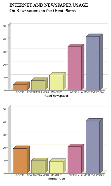
Conclusions:
Residents in the target population are as likely to use the Internet daily for information as to read a daily newspaper.
There is no correlation between Internet use and traditional media use.
SCENARIO 3: PROGRAM EVALUATION
In the previous scenarios, the variables to be used were already identified and it was assumed that whatever measure being used was reliable and valid. In evaluations of specific programs or products, this assumption cannot always be made.
In this example, a test comprised of multiple choice questions and short case studies was developed by the client and used for the first time in this evaluation. No assumptions can be made and we need to begin by testing everything from whether there are gross data entry errors to internal consistency reliability. This is before we get to answer the client’s question, which was whether the two-day staff training program was effective.
Just for fun, I decided to complete the whole project using only two procedures.
Wonder of SAS: One step produces multiple steps in psychometric analysis
Not coincidentally, the WHERE statement below illustrates a point that should be familiar by now – know your data! An assumption of most statistical tests is that the data are independent, random observations. If pre- and the post-tests of the same people are included, this assumption is grossly violated.
PROC CORR DATA = tests ALPHA ;
WHERE test_type = “pre” ;
VAR q1 – – q40 ;
Descriptive statistics, which the CORR procedure produces by default, include the
minimum and maximum for every variable, which are checked to make sure that nothing is out of range. Nothing is less than zero or greater than the maximum allowable points for that item. All of the items are at least within range.
Next step, as any good psychometrician knows is to examine the item means and variances. If there is any question that everyone got wrong (mean = 0) , or that everyone got right, then it will have a variance of zero. These items would bear further examination, but there aren’t any on this test.
Coefficient alpha is a measure of the internal consistency reliability of the test. The .67 value is undesirably low. This analysis shows several items that have a negative correlation with the total, which is inconsistent with the assumption that all items measure the same thing, i.e. knowledge of regulations, specific concepts and best practices applying to the jobs these individuals do. Answering an item correctly should not be negatively related to the total score.
Possibly two different factors are being measured. Maybe these items that are negatively correlated with the total are all measuring some other trait – compliance or social appropriateness – that is perhaps negatively related to staff effectiveness.
The correlation matrix, also produced in the same step, is scrutinized to determine whether these items negatively correlated with the total score perhaps correlate with each other. It seems that these are just bad items. As we examine them, they ask questions like “Which of these is a website where you could look up information on …..” which may be a measure of how much time you spend at work goofing off searching the Internet.
Having verified that no data are out of range, gone back to a DATA step , deleted bad items to produce a scale with acceptable reliability and used a SUM function to create a total score for each person, pre- training and post-training, it is time for the next step.
Wonder of SAS: The General Linear Model Really is General
A valid measure of employee skills should be related to job-specific education, but not to age. To determine how much the test score initially was determined by education and age one could use a PROC REG but I decided to use Proc GLM because it is the General Linear Model and, after all, regression is a special case of the general model.
TITLE “Regression” ;
PROC GLM DATA=in.test2 ;
MODEL score = age years_of_ed ;
WHERE test_type = “pre” ;
The focus of the training was on care for people with chronic illness. Perhaps if a person had a chronic illness him/herself or had previous experience in a job providing such care it would be related to their pre-existing knowledge.
This is an obvious 2 x 2 Analysis of Variance, which can be done with a Proc GLM, because, of course, Analysis of Variance is another special case of the General Linear Model. So, I did it.
TITLE “2 x 2 Analysis of Variance ” ;
PROC GLM DATA=in.test2 ;
CLASS disability job;
MODEL score = disability job disability*job ;
WHERE test_type = “pre” ;
Whether or not a subject had disability was unrelated to the score but experience on the job was. The test has adequate reliability, some evidence for validity.
The real question of interest is whether scores increased from pre- to post-test for the experimental group but not the control group. For this I am going to use, of course, the General Linear Model for a repeated measures ANOVA
TITLE “Repeated Measures Analysis of Variance ” ;
PROC GLM DATA = in.mrgfiles ;
CLASS test_group ;
MODEL score score2 = test_group ;
REPEATED test 2 ;
LSMEANS test_group ;
It can be seen that the model is highly significant, that there is a significant interaction of test * test_group, exactly as hoped, and the output from the LSMEANS statement provides the welcome information that the trained group increased its score from 45% to 68% while the comparison group score only showed an increase of less than 2% – from 57.4% to 59%.
CONCLUSION
SAS has made it possible for thousands of people to obtain output of statistical procedures without ever needing to understand the assumptions of independently sampled random data, what an F distribution is, the impact of measurement error on correlation obtained or even what error variance is. This is a mixed blessing as ERROR-free logs in no way guarantee error-free results or interpretation.
On the other hand, SAS, particularly with the Enterprise Guide, has made great progress in making statistics accessible to a wider audience and perhaps moved more statisticians to understand that the best statistical analysis is not the one that the fewest people can understand but that the most people can understand. So far, I can’t find anything bad about that.
Contact information:
AnnMaria DeMars
University of Southern California
Information Technology Services, Customer Support Center
Los Angeles, CA
ademars@usc.edu
(213) 740-2840
Hi,
Very interesting paper.
I suggest you create RSS feed for you blog, so that others can browse your log easilier. 🙂
Great tips, especially #2 on survey(stratification). Keep the blogs coming.