Variance and Eigenvalues
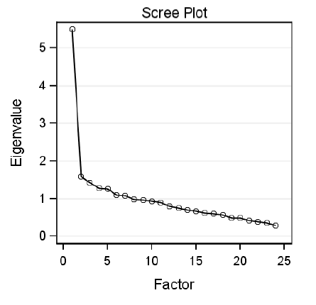
I find this scree plot of eigenvalues very helpful in identifying the number of factors. A scree plot is a plot of the eigenvalues by the factor number.
I realized this is only helpful if one understands what an eigenvalue is.
 First of all, go way back to Stat 101 & remember that correlation is the covariance of z-scores which have a standard deviation of 1, and since the square of 1 = 1, they also have a variance of 1
Understand that the default is to factor analyze the correlation matrix and that means that your variables are standardized before analysis, with a variance of 1. So, that is the total amount of variance we are trying to explain for each variable.
Therefore, the total amount of variance to be explained in a matrix will equal the number of variables. If you have 10 variables, the total amount of variance to be explained is 10.
If you’ve ever looked a correlation matrix you will have noticed that all of the diagonals are 1. The correlation of an item with itself is 1.
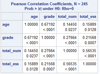 What percentage of the variance in an item is explained by itself? It should be obvious that it is 100%. If I know your age, for example, I can predict your age with 100% accuracy. Duh.
An eigenvalue is the total amount of variance in the variables in the dataset explained by the common factor. (Mathematically, it’s the sum of the squared factor loadings. If you are interested in that, you can come to my class at WUSS on Wednesday morning. Or, possibly, I’ll blog about it next week.)
Now, if a factor has an eigenvalue of 1, it is pretty useless. That is because the whole purposes of factor analysis is to replace your 20 or 50 items that each explain of variance of 1 (their own variance) with a few common factors. A factor with an eigenvalue of 1 doesn’t explain any more variance than a single item.
Let’s say you have 24 items and your first factor has an eigenvalue of 6. Is that good? Yes, because that means that a single factor explains as much of the variance in the matrix of data as six items. If you could get four orthogonal factors, each with an eigenvalue close to 6, then you would have explained nearly 100% of the variance in your 24 items with just 4 factors.
Think about correlation matrices again. It’s not often you see an EXACTLY zero correlation. You’ll find correlations of .08, .03, .12 just by chance. Who knows, the same person had the highest score on sticks of bubble gum chewed and number of asses kicked (R.I.P. Rowdy Roddy Piper), it doesn’t mean that those two variables really have that much in common. This is why we look at statistical significance and how likely something is to occur by chance.
How do you tell if that factor has a higher degree of common variance, that is the eigenvalue is higher, than would be expected by chance? One way is the scree plot. You look at the eigenvalue for each factor and see where it drops off.
I would write more about this but my family is urging me to leave for a barbecue for Maria’s birthday, so you will have to last until tomorrow for a more detailed explanation of scree plots and why they are called that.
——-
Random act of advertising: Buy our games – learn history, learn math, find herbs, spear fish

If you want to be really cool and get a Tourist Visa to our Virtual Worlds, you can apply here.
Very through, concise, easily understood explanation of eigenvalue. Thank you. Intending to use Factominer, an R capability to do MCA on a set of data with 4500 variables, most columns only have a small sub-set of those variables. Not certain that Factominer can provide discernable results, we’ll see. If you’re interested, I’ll share results with you.
Again, thanks for an interesting post, hope your cook-out went well.
thank you so much. i was struggling to understand it. this totally cleared it for me