MANOVA from beginning to end : Creating the scales

Last time, we saw how to recode variables to score answers correct or incorrect, on a rating scale and weighted by importance. Today, we’re going to look at creating some scales from those variables because for reasons I’m sure I have written about at some point in the past, single items are usually not very reliable. Whether you use SAS, SPSS, R or any other statistical package, you are still going  to need to follow the steps of recoding your variables and creating and validating your scales before you get into MANOVA. Or, at least, you will if you are smart.

First, I want to check that there are no obvious errors or other problems in my data.
PROC MEANS DATA=example ;
VAR gr2A -- gr39 hbs1 --d_gr12a ;

You could type in the variable names but that is a lot of typing. The double dashes mean to include all variables in the data set in order from the first variable to the one that comes after the dashes. How do you know what order the variables are in? Click on the OUTPUT DATA tab at the top and look to the left under COLUMNS.

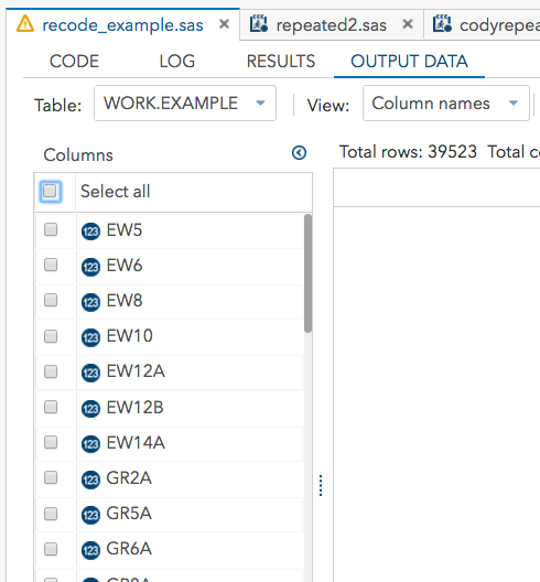
If you didn’t just run a program creating your data and hence don’t have an OUTPUT DATA tab, you can find your data file by clicking the MY LIBRARIES tab and then clicking on the library (directory) where your data are kept and clicking on the dataset to open it. You can also use the PROC CONTENTS procedure but today we are being all pointy and clicky with SAS Studio.

Sometimes you will see something like:

VAR item1 – item12 ;

The single dash is used for variables that end in a number and if you don’t have item1, item2 all the way through item12, it will give you an error and not run. Then you will be sad.

PROC MEANS will give you the N, mean, standard deviation, minimum and maximum.

Here are a few things to consider.

• Is the N substantially less than you had expected? If so, you have a lot of missing data and you should investigate that. The lowest N I have is 37, 814 out of 39, 430 people so not bad, but I might want to look at that one item, since most of the items have close to 39,000 for an N
• Is your standard deviation zero? STOP RIGHT THERE!  On just what variable could 39,000 people give the same response? This likely shows a big problem with your data. I did not have that problem, so I continued.
• Are your minimum and maximum the minimum and maximum possible scores for the item? Now, this may not always be the case. On a scale of 1 to 10, say, with a sample of 50 people, maybe no one will say 1. However, I have over 39,000 people and the items are 0 or 1, o – 2  or 1- 3, so I should have people from the minimum to the maximum or something is wrong. Nothing is wrong, and I continue.
• Are the means about what you expect? Well, I’m not really an expert on social structure and family relations in India, so I can’t say. About a third of the women said it was usual for a husband to beat his wife if her dowry was not what was expected. About three-fourths said they would be allowed to visit a family or friend’s home alone.

Okay, so my results from the means procedure looks okay. Now what?

Next, I’m going to do a factor analysis to see if my supposition is supported of three scales related to health, beating your wife and autonomy.

Here is the code for my factor analysis.

PROC FACTOR DATA =example SCREE ROTARE= VARIMAX NFACTORS=5;
VAR gr2A -- gr39 hbs1 --d_gr12a ;

This is actually the second one I ran. In inspecting the results for the first, between the eigenvalues and scree plot, I decided that at most I should retain five factors. I’ve written a lot about factor analysis on this blog previously, so I’m not going to go into detail here.  In short, the decision-making variables mostly loaded on the first factor with factor loadings of .70 and higher. The median communality estimate for those items was about .67.  In short, considerable evidence for a decision-making factor. The wife-beating variables loaded on the second factor. All but one loaded above .67, and even that variable (Beating your wife if she had an extramarital affair – which 84% of the women said was accepted in their communities) loaded at .40. The variables regarding needing permission to go places loaded on the third factor and also had high communality estimates. The variables regarding going places by yourself loaded on the fourth factor and also had high communality estimates.

The health variables were a different story. Four out of six loaded between .47 and .67 on the fifth factor. The other two did not load on any factor.

It is starting to look like at this point that it is okay to retain the wife-beating items as a scale. The various measures of autonomy  – decision-making, going places on your own and needing permission – seem to hang together within factors. I think it would be reasonable to put all three of these together in one scale. I talked about parceling in the past, and I could have done that as a step here, and then re-run the factor analysis to support (or not) my supposed autonomy factor. Since I have limited time and simply doing this analysis for educational and illustrative purposes, I skipped over this to the next procedure, which is reliability analysis.

Since this post is pretty long already, I’ll save that for the next post.

When I am not writing about statistics, I’m making games that teach math, social studies and language.

Check them out.