MANOVA from beginning to end: Reliability
 Where is the Multivariate Analysis of Variance ?
You promised there would be MANOVA ! Now we’re in the third post!
First there was recoding of variables.
Then, there was creating scales.
Now, we’re looking at reliability.
Patience is a virtue.
Before we get to doing a MANOVA we want to be sure that our dependent and independent variables are reliable and valid. Let’s move on to reliability.
I’m going to do a correlation matrix and a Cronbach alpha, which is a measure of internal consistency. The rationale is that if items all measure the same construct – say, knowledge of health practices, or autonomy or acceptance of wife beating – then those items should be related to one another. An alpha of 0 would indicate the covariance of items in the scale are zero, so, your scale sucks. An alpha of .95 would mean your scale is amazingly consistent.
So, I did three analysis for my three scales
Title "Health Variables " ;

proc corr data=example alpha ;

var hbs1 hbs3-hbs7 ;
Title "Wife beating variables" ;

proc corr data=example alpha ;

var GR34 - GR39 ;
Title "Decision Variables" ;

proc corr data=example alpha ;

VAR D_GR1A GR2A D_GR3A D_GR4A GR5a GR6A D_GR7A GR8A

D_GR9A GR9F D_GR10A D_GR12A GR10F GR12F ;
Let’s skip the simple statistics, mean, etc. you get from these analyses and go to the alpha
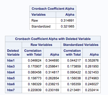
The alpha for the health scale is pretty bad. The value for the raw scores is .31, for standardized items, still really bad at .32. When we look at how deleting a variable would improve the alpha, if we dropped the first variable , the alpha would go up to .34 – but that is still awful.
For the wife-beating scale the raw value for alpha was .81 and also for the standardized value. So, that one was pretty good as far as reliability.
I put all of the decision variables together, the ones on whether the woman was involved in making decisions, could go places on her own, needed to ask permission to go places. The Cronbach alpha for the raw variables was .65, for standardized variables .81. Note that standardized variables are placed on the same metric, so my idea of some variables being much more important than others did not pan out.
So … I standardized the variables, then I read in that data set and created two scales, one that was a sum of the decision variables and the other that was the mean of the 6 wife-beating variables. There was no particular reason for using the mean of the six variables as opposed to just adding them up. I did both methods to show it was an option.
BEWARE THE SUM FUNCTION – Note, I did not use the sum function. If you add up the values, as shown below, and one of the variables has a missing value then the value of the sum is going to be missing. If you used the SUM function, the variables that have non-missing values would be added up, so the missing value would be treated as a zero. There are times where that is acceptable. This is not one of those times.
While I’m at it, I want to check whether the scales have approximately normal distributions. A perfectly normal distribution would have skewness and kurtosis values of 0.
proc standard data=example mean=0 std=1 out=MAN_data;
Data create_manova ;

set man_data ;

* I could have used the mean function here, but I didn't ;

decision = D_GR1A + GR2A + D_GR3A + D_GR4A + GR5a + GR6A + D_GR7A + GR8A +

D_GR9A + GR9F + D_GR10A + D_GR12A + GR10F + GR12F ;

beating = mean(of gr34-gr39);
proc univariate data=create_manova ;

var decision beating ;
The skewness values were relatively low: -1.3 and 0.2 for the two scales and kurtosis values were 2.0 and -1.2 . Since my scales aren’t a radical departure from normality, I’m now going on to MANOVA – finally!