How to write a statistical analysis paper: Step Three

So far, we have looked at

1. How to get the sample demographics and descriptive statistics for your dependent and independent variable.
2. Computing descriptive statistics by category 

Now it’s time to dive into step 3, computing inferential statistics.

The code is quite simple. We need a LIBNAME statement. It will look something like this. The exact path to the data, which is between the quotation marks, will be different for every course. You get that path from your professor.

LIBNAME mydata “/courses/ab1234/c_0001/” access=readonly;

DATA example ;
SET mydata.coh602;
WHERE race ne “” ;
run ;

I’m creating a data set named example. The DATA statement does that.

It is being created as a subset from the coh602 dataset stored in the library referenced by mydata. The SET statement does that.

I’m only including those records where they have a non-missing value for race. The WHERE statement does that.

If you already did that earlier in your program, you don’t need to do it again. However, remember, example is a temporary data set (you can tell because it doesn’t have a two level name like mydata.example ) . It resides in working memory. Think of it as if you were working on a document and didn’t save it. If you closed that application, your document would be gone.  Okay, so much for the data set. Now we are on to ….. ta da da

Inferential Statistics Using SAS

Let’s start with Analysis of Variance.  We’re going to do PROC GLM. GLM stands for General Linear Model. There is a PROC ANOVA also and it works pretty much the same.

PROC GLM DATA = example ;

CLASS race ;

MODEL bmi_p = race ;

MEANS race / TUKEY ;

The CLASS statement is used to identify any categorical variables. Since with Analysis of Variance you are comparing the means of multiple groups, you need at least one CLASS statement with at least one variable that has multiple groups – in this case, race.

MODEL dependent = independent ;

Our model is of bmi_p  – that is body mass index, being dependent on race. Your dependent variable MUST be a numeric variable.

The model statement above will result in a test of significance of difference among means and produce an F-statistic.

What does an F-test test?

It tests the null hypothesis that there is NO difference among the means of the groups, in this case, among the three groups – White, Black and Hispanic . If the null hypothesis is accepted, then all the group means are the same and you can stop.

However, if the null hypothesis is rejected, you certainly also want to know which groups are different from which other groups. After that significant F-test, you need a post hoc test (Latin for “after that”. Never say all those years of Catholic school were wasted).

There are a lot to choose from but for this I used TUKEY. The last statement requests the post hoc test.

Let’s take a look at our results.

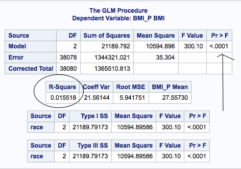
I have an F-value of 300.10 with a probability < .0001 .

Assuming my alpha level was .o5 (or .01, or .001, or .ooo1) , this is statistically significant and I would reject my null hypothesis. The differences between means are probably not zero, based on my F-test, but are they anything substantial?

If I look at the R-square, and I should, it tells me that this model explains 1.55% of the variance in BMI – which is not a lot. The mean BMI for the whole sample is 27.56.

You can see complete results here. Also, that link will probably work better with screen readers, if you’re visually impaired (Yeah, Tina, I put this here for you!).

 

Next, I want to look at the results of the TUKEY test.

 

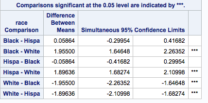
We can see that there was about a 2-point difference between Blacks and Whites, with the mean for Blacks 2 points higher. There was also about a 2-point difference between Whites and Hispanics. The difference in mean BMI between White and Black samples and White and Hispanic samples was statistically significant. The difference between Hispanic and Black sample means was near zero with the mean BMI for Blacks 0.06 points higher than for Hispanics.

This difference is not significant.

So …. we have looked at the difference in Body Mass Index, but is that the best indicator of obesity? According to the World Health Organization, who you’d think would know, obesity is defined as a BMI of greater than 30.

The next step we might want to take is examine our null hypothesis using categorical variable, obese or not obese. That, is our next analysis and next post.